Orange Juice
Data Mining and Business Analytics with R
This is an example presented in the book “Data Mining and Business Analytics with R”, with some useful basic graphs that can be reused for other sets of similar data. Code and Data are saved in Github link
store     brand week   logmove feat price     AGE60      EDUC    ETHNIC   INCOME   HHLARGE
1      2 tropicana   40  9.018695    0  3.87 0.2328647 0.2489349 0.1142799 10.55321 0.1039534
2      2 tropicana   46  8.723231    0  3.87 0.2328647 0.2489349 0.1142799 10.55321 0.1039534
3      2 tropicana   47  8.253228    0  3.87 0.2328647 0.2489349 0.1142799 10.55321 0.1039534
4      2 tropicana   48  8.987197    0  3.87 0.2328647 0.2489349 0.1142799 10.55321 0.1039534
5      2 tropicana   50  9.093357    0  3.87 0.2328647 0.2489349 0.1142799 10.55321 0.1039534
6      2 tropicana   51  8.877382    0  3.87 0.2328647 0.2489349 0.1142799 10.55321 0.1039534
7      2 tropicana   52  9.294682    0  3.29 0.2328647 0.2489349 0.1142799 10.55321 0.1039534
8      2 tropicana   53  8.954674    0  3.29 0.2328647 0.2489349 0.1142799 10.55321 0.1039534
9      2 tropicana   54  9.049232    0  3.29 0.2328647 0.2489349 0.1142799 10.55321 0.1039534
10     2 tropicana   57  8.613230    0  3.29 0.2328647 0.2489349 0.1142799 10.55321 0.1039534
11     2 tropicana   58  8.680672    0  3.56 0.2328647 0.2489349 0.1142799 10.55321 0.1039534
12     2 tropicana   59  9.034080    0  3.56 0.2328647 0.2489349 0.1142799 10.55321 0.1039534
13     2 tropicana   60  8.691483    0  3.56 0.2328647 0.2489349 0.1142799 10.55321 0.1039534
14     2 tropicana   61  8.831712    0  3.56 0.2328647 0.2489349 0.1142799 10.55321 0.1039534
15     2 tropicana   62  9.128696    0  3.87 0.2328647 0.2489349 0.1142799 10.55321 0.1039534
16     2 tropicana   63  9.405907    0  2.99 0.2328647 0.2489349 0.1142799 10.55321 0.1039534
17     2 tropicana   64  9.447150    0  2.99 0.2328647 0.2489349 0.1142799 10.55321 0.1039534
18     2 tropicana   65  8.783856    0  3.59 0.2328647 0.2489349 0.1142799 10.55321 0.1039534
19     2 tropicana   66  8.723231    0  3.59 0.2328647 0.2489349 0.1142799 10.55321 0.1039534
20     2 tropicana   67  9.957976    0  2.39 0.2328647 0.2489349 0.1142799 10.55321 0.1039534
21     2 tropicana   68  9.426741    0  2.39 0.2328647 0.2489349 0.1142799 10.55321 0.1039534
22     2 tropicana   69  9.156095    0  3.59 0.2328647 0.2489349 0.1142799 10.55321 0.1039534
23     2 tropicana   70  9.793673    0  2.59 0.2328647 0.2489349 0.1142799 10.55321 0.1039534
24     2 tropicana   71  9.149316    0  2.59 0.2328647 0.2489349 0.1142799 10.55321 0.1039534
25     2 tropicana   72  8.743851    0  3.59 0.2328647 0.2489349 0.1142799 10.55321 0.1039534
26     2 tropicana   73  8.841014    0  3.59 0.2328647 0.2489349 0.1142799 10.55321 0.1039534
27     2 tropicana   74  9.727228    0  2.49 0.2328647 0.2489349 0.1142799 10.55321 0.1039534
28     2 tropicana   75  8.743851    0  3.59 0.2328647 0.2489349 0.1142799 10.55321 0.1039534
29     2 tropicana   76  8.979165    0  3.59 0.2328647 0.2489349 0.1142799 10.55321 0.1039534
30     2 tropicana   77  8.723231    0  3.59 0.2328647 0.2489349 0.1142799 10.55321 0.1039534
31     2 tropicana   78  8.979165    0  3.59 0.2328647 0.2489349 0.1142799 10.55321 0.1039534
32     2 tropicana   79  8.962904    0  3.59 0.2328647 0.2489349 0.1142799 10.55321 0.1039534
33     2 tropicana   80  8.712760    0  3.59 0.2328647 0.2489349 0.1142799 10.55321 0.1039534
34     2 tropicana   81 10.649607    1  1.69 0.2328647 0.2489349 0.1142799 10.55321 0.1039534
35     2 tropicana   82  8.502689    0  3.59 0.2328647 0.2489349 0.1142799 10.55321 0.1039534
36     2 tropicana   83 10.292281    1  1.99 0.2328647 0.2489349 0.1142799 10.55321 0.1039534
37     2 tropicana   84  9.208739    0  3.59 0.2328647 0.2489349 0.1142799 10.55321 0.1039534
38     2 tropicana   85 10.468801    1  1.99 0.2328647 0.2489349 0.1142799 10.55321 0.1039534
39     2 tropicana   86 10.083139    0  1.99 0.2328647 0.2489349 0.1142799 10.55321 0.1039534
40     2 tropicana   87  8.868413    0  3.59 0.2328647 0.2489349 0.1142799 10.55321 0.1039534
41     2 tropicana   88 10.106918    1  2.29 0.2328647 0.2489349 0.1142799 10.55321 0.1039534
42     2 tropicana   89  8.754003    0  3.59 0.2328647 0.2489349 0.1142799 10.55321 0.1039534
43     2 tropicana   90  8.712760    0  3.59 0.2328647 0.2489349 0.1142799 10.55321 0.1039534
44     2 tropicana   91 10.420375    0  1.99 0.2328647 0.2489349 0.1142799 10.55321 0.1039534
45     2 tropicana   92  9.491602    0  1.99 0.2328647 0.2489349 0.1142799 10.55321 0.1039534
46     2 tropicana   93  8.733594    0  3.59 0.2328647 0.2489349 0.1142799 10.55321 0.1039534
47     2 tropicana   94  9.270871    0  3.59 0.2328647 0.2489349 0.1142799 10.55321 0.1039534
48     2 tropicana   95 10.707102    0  1.99 0.2328647 0.2489349 0.1142799 10.55321 0.1039534
49     2 tropicana   97  9.908276    0  1.99 0.2328647 0.2489349 0.1142799 10.55321 0.1039534
50     2 tropicana   98  9.121728    1  3.59 0.2328647 0.2489349 0.1142799 10.55321 0.1039534
51     2 tropicana   99  9.996614    0  2.19 0.2328647 0.2489349 0.1142799 10.55321 0.1039534
52     2 tropicana  100  9.515469    0  2.19 0.2328647 0.2489349 0.1142799 10.55321 0.1039534
53     2 tropicana  103  8.333270    0  3.59 0.2328647 0.2489349 0.1142799 10.55321 0.1039534
54     2 tropicana  104 10.582130    1  1.99 0.2328647 0.2489349 0.1142799 10.55321 0.1039534
55     2 tropicana  105  8.636220    0  3.59 0.2328647 0.2489349 0.1142799 10.55321 0.1039534
56     2 tropicana  106  9.107643    1  2.68 0.2328647 0.2489349 0.1142799 10.55321 0.1039534
57     2 tropicana  107  8.702178    0  3.44 0.2328647 0.2489349 0.1142799 10.55321 0.1039534
58     2 tropicana  108  8.954674    0  3.14 0.2328647 0.2489349 0.1142799 10.55321 0.1039534
     WORKWOM   HVAL150 SSTRDIST  SSTRVOL CPDIST5   CPWVOL5
1  0.3035853 0.4638871 2.110122 1.142857 1.92728 0.3769266
2  0.3035853 0.4638871 2.110122 1.142857 1.92728 0.3769266
3  0.3035853 0.4638871 2.110122 1.142857 1.92728 0.3769266
4  0.3035853 0.4638871 2.110122 1.142857 1.92728 0.3769266
5  0.3035853 0.4638871 2.110122 1.142857 1.92728 0.3769266
6  0.3035853 0.4638871 2.110122 1.142857 1.92728 0.3769266
7  0.3035853 0.4638871 2.110122 1.142857 1.92728 0.3769266
8  0.3035853 0.4638871 2.110122 1.142857 1.92728 0.3769266
9  0.3035853 0.4638871 2.110122 1.142857 1.92728 0.3769266
10 0.3035853 0.4638871 2.110122 1.142857 1.92728 0.3769266
11 0.3035853 0.4638871 2.110122 1.142857 1.92728 0.3769266
12 0.3035853 0.4638871 2.110122 1.142857 1.92728 0.3769266
13 0.3035853 0.4638871 2.110122 1.142857 1.92728 0.3769266
14 0.3035853 0.4638871 2.110122 1.142857 1.92728 0.3769266
15 0.3035853 0.4638871 2.110122 1.142857 1.92728 0.3769266
16 0.3035853 0.4638871 2.110122 1.142857 1.92728 0.3769266
17 0.3035853 0.4638871 2.110122 1.142857 1.92728 0.3769266
18 0.3035853 0.4638871 2.110122 1.142857 1.92728 0.3769266
19 0.3035853 0.4638871 2.110122 1.142857 1.92728 0.3769266
20 0.3035853 0.4638871 2.110122 1.142857 1.92728 0.3769266
21 0.3035853 0.4638871 2.110122 1.142857 1.92728 0.3769266
22 0.3035853 0.4638871 2.110122 1.142857 1.92728 0.3769266
23 0.3035853 0.4638871 2.110122 1.142857 1.92728 0.3769266
24 0.3035853 0.4638871 2.110122 1.142857 1.92728 0.3769266
25 0.3035853 0.4638871 2.110122 1.142857 1.92728 0.3769266
26 0.3035853 0.4638871 2.110122 1.142857 1.92728 0.3769266
27 0.3035853 0.4638871 2.110122 1.142857 1.92728 0.3769266
28 0.3035853 0.4638871 2.110122 1.142857 1.92728 0.3769266
29 0.3035853 0.4638871 2.110122 1.142857 1.92728 0.3769266
30 0.3035853 0.4638871 2.110122 1.142857 1.92728 0.3769266
31 0.3035853 0.4638871 2.110122 1.142857 1.92728 0.3769266
32 0.3035853 0.4638871 2.110122 1.142857 1.92728 0.3769266
33 0.3035853 0.4638871 2.110122 1.142857 1.92728 0.3769266
34 0.3035853 0.4638871 2.110122 1.142857 1.92728 0.3769266
35 0.3035853 0.4638871 2.110122 1.142857 1.92728 0.3769266
36 0.3035853 0.4638871 2.110122 1.142857 1.92728 0.3769266
37 0.3035853 0.4638871 2.110122 1.142857 1.92728 0.3769266
38 0.3035853 0.4638871 2.110122 1.142857 1.92728 0.3769266
39 0.3035853 0.4638871 2.110122 1.142857 1.92728 0.3769266
40 0.3035853 0.4638871 2.110122 1.142857 1.92728 0.3769266
41 0.3035853 0.4638871 2.110122 1.142857 1.92728 0.3769266
42 0.3035853 0.4638871 2.110122 1.142857 1.92728 0.3769266
43 0.3035853 0.4638871 2.110122 1.142857 1.92728 0.3769266
44 0.3035853 0.4638871 2.110122 1.142857 1.92728 0.3769266
45 0.3035853 0.4638871 2.110122 1.142857 1.92728 0.3769266
46 0.3035853 0.4638871 2.110122 1.142857 1.92728 0.3769266
47 0.3035853 0.4638871 2.110122 1.142857 1.92728 0.3769266
48 0.3035853 0.4638871 2.110122 1.142857 1.92728 0.3769266
49 0.3035853 0.4638871 2.110122 1.142857 1.92728 0.3769266
50 0.3035853 0.4638871 2.110122 1.142857 1.92728 0.3769266
51 0.3035853 0.4638871 2.110122 1.142857 1.92728 0.3769266
52 0.3035853 0.4638871 2.110122 1.142857 1.92728 0.3769266
53 0.3035853 0.4638871 2.110122 1.142857 1.92728 0.3769266
54 0.3035853 0.4638871 2.110122 1.142857 1.92728 0.3769266
55 0.3035853 0.4638871 2.110122 1.142857 1.92728 0.3769266
56 0.3035853 0.4638871 2.110122 1.142857 1.92728 0.3769266
57 0.3035853 0.4638871 2.110122 1.142857 1.92728 0.3769266
58 0.3035853 0.4638871 2.110122 1.142857 1.92728 0.3769266
 [ reached 'max' / getOption("max.print") -- omitted 28889 rows ]
## Install packages from CRAN; use any USA mirror
library(lattice)
#oj <- read.csv("https://www.biz.uiowa.edu/faculty/jledolter/DataMining/oj.csv")
oj <- read.csv("oj.csv")
oj$store <- factor(oj$store) #change numberic value of store into categorical data
oj[1:2,]
t1=tapply(oj$logmove,oj$brand,FUN=mean,na.rm=TRUE) #calculate the mean of each brand using logmove value.
t1
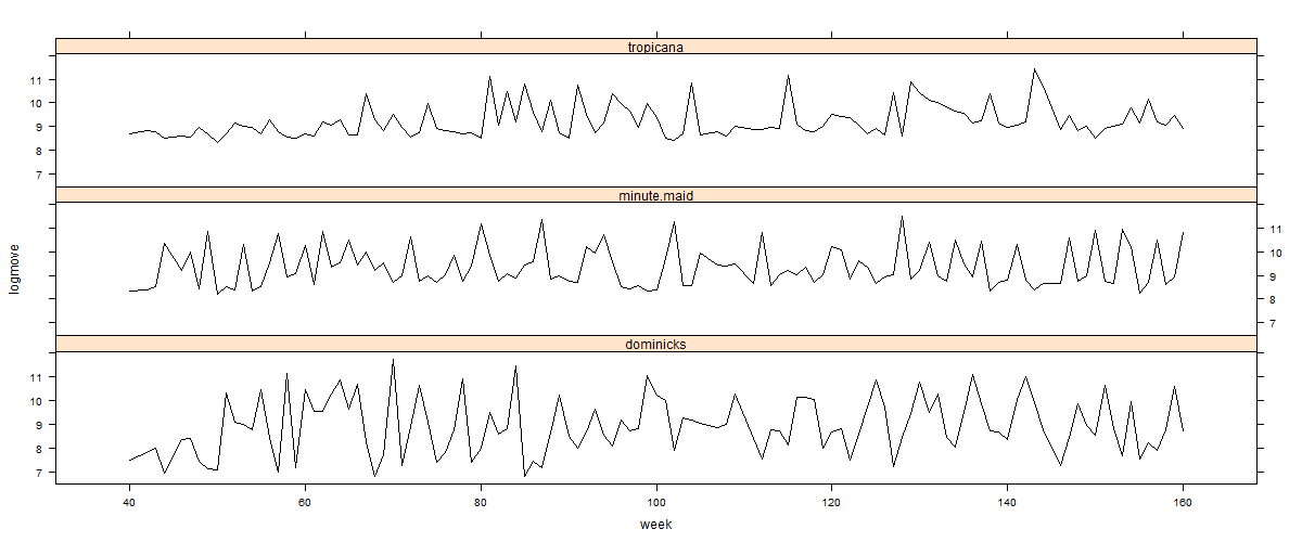
t2=tapply(oj$logmove,INDEX=list(oj$brand,oj$week),FUN=mean,na.rm=TRUE) #calculate the mean of logmove value based on index lists per week.
t2
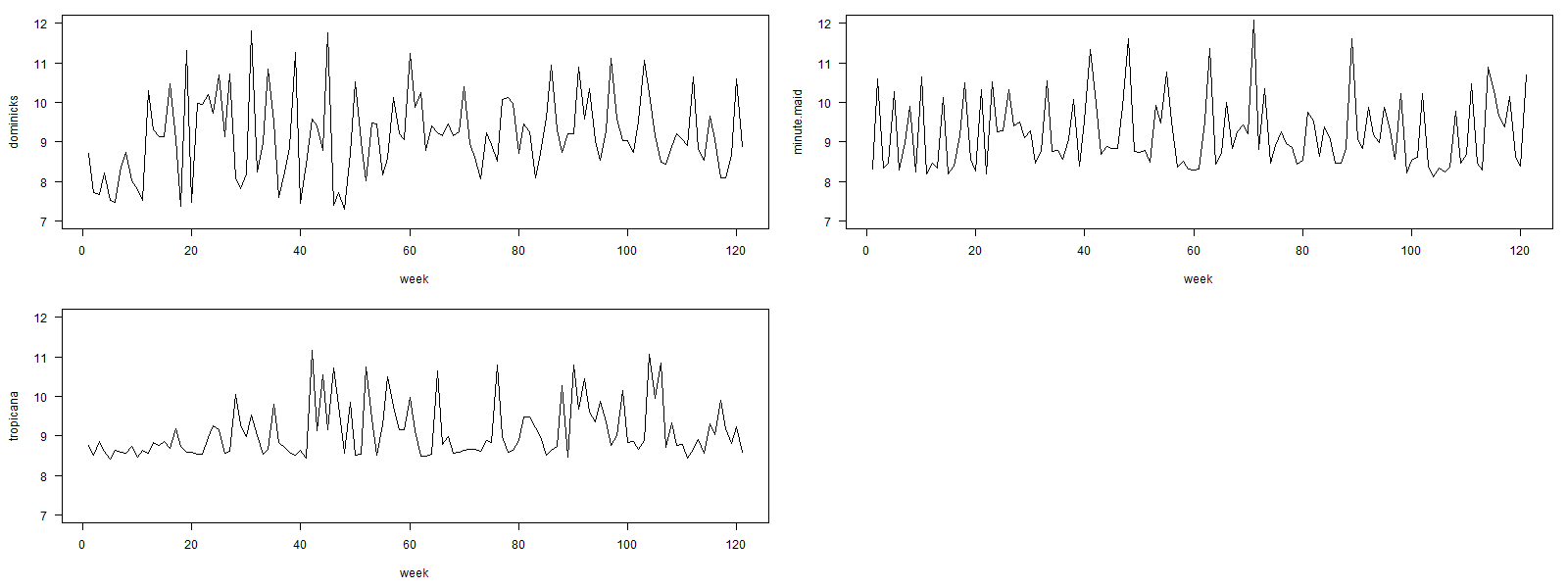
#plot each graph as time serieas data per week.
plot.new()
par(mar=c(4.5,4.3,1,1)+0.1,mfrow=c(2,2),bg="white",cex = 1, cex.main = 0.6)
plot(t2[1,],type= "l",xlab="week",ylab="dominicks",ylim=c(7,12),cex.axis = 1,las = 1)
plot(t2[2,],type= "l",xlab="week",ylab="minute.maid",ylim=c(7,12),cex.axis = 1,las = 1)
plot(t2[3,],type= "l",xlab="week",ylab="tropicana",ylim=c(7,12),cex.axis = 1,las = 1)
dev.copy(png,'oj_weekmean01.png',width = 1600, height = 600)
dev.off()
#-------------------------------
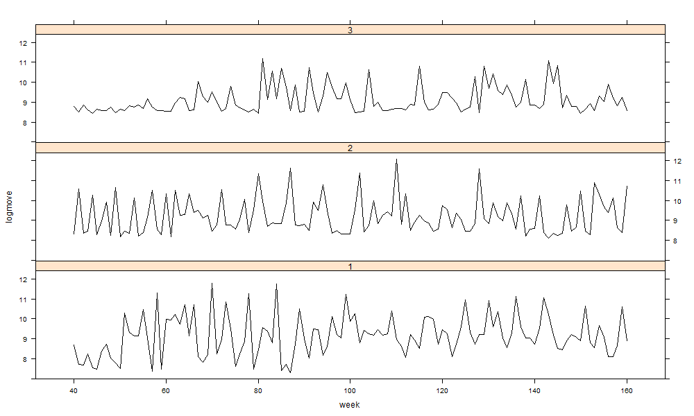
#now we combine the three above graphs into one single graphs for ease of comparison
logmove=c(t2[1,],t2[2,],t2[3,])
week1=c(40:160)
week=c(week1,week1,week1)
brand1=rep(1,121)
brand2=rep(2,121)
brand3=rep(3,121)
brand=c(brand1,brand2,brand3)
plot.new()
xyplot(logmove~week|factor(brand),type= "l",layout=c(1,3),col="black")
dev.copy(png,'oj_weekmean02.png',width = 1000, height = 600)
dev.off()
#-----------------------------
plot.new()
par(mfrow=c(1,1))
#par(mar=c(4.5,4.3,1,1)+0.1,mfrow=c(2,2),bg="white",cex = 1, cex.main = 0.6)
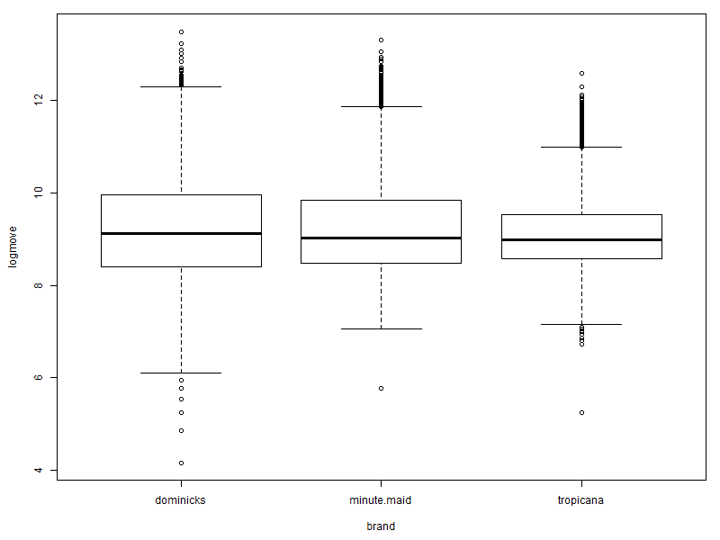
boxplot(logmove~brand,data=oj) # compare logmove of 3 branch using boxplot
dev.copy(png,'oj_logmovebrandboxplot.png',width = 800, height = 600)
dev.off()
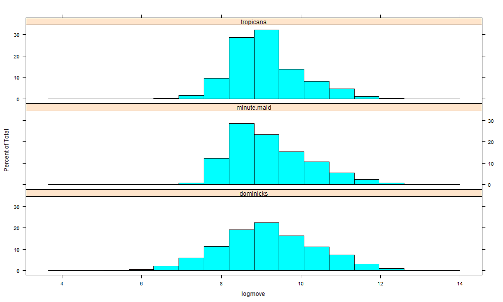
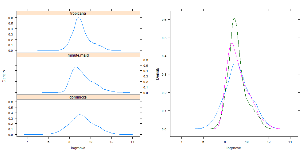
histogram(~logmove|brand,data=oj,layout=c(1,3)) # compare logmove of 3 branch using histogram
dev.copy(png,'oj_logmovebrandhist.png',width = 1000, height = 600)
dev.off()
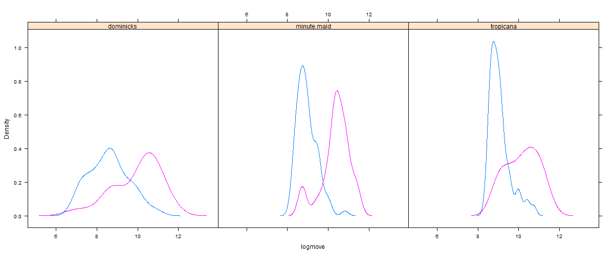
a1=densityplot(~logmove|brand,data=oj,layout=c(1,3),plot.points=FALSE) # compare logmove of 3 branch using density plot
a2=densityplot(~logmove,groups=brand,data=oj,plot.points=FALSE) ## compare logmove of 3 branch using density plot in a one frame
#using xyplot to see the spartial distribution of data weekly
library(gridExtra) #this package allows to plot multiple graphs in the same plot despite the difference in plotting engines (e.g. ggplot or barchart)
grid.arrange(a1, a2, ncol = 2) #display the two plot a and p
dev.copy(png,'oj_logmovedensity.png',width = 1000, height = 500)
dev.off()
#-------------------------------------------------
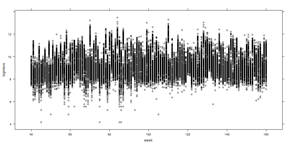
xyplot(logmove~week,data=oj,col="black")
dev.copy(png,'oj_logmoveweekspartial.png',width = 1000, height = 500)
dev.off()
#---------------------------------
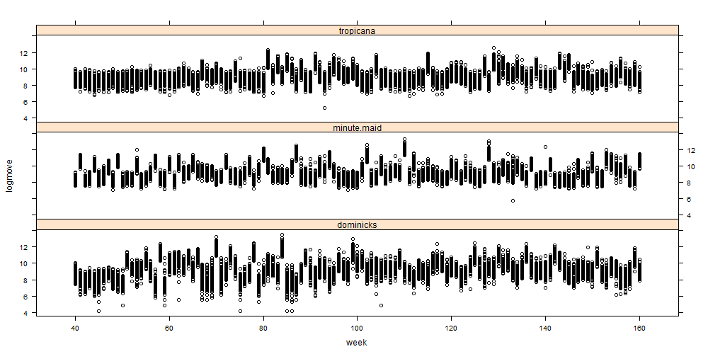
xyplot(logmove~week|brand,data=oj,layout=c(1,3),col="black")
dev.copy(png,'oj_logmoveweekspartialbrand.png',width = 1000, height = 500)
dev.off()
#---------------------------------
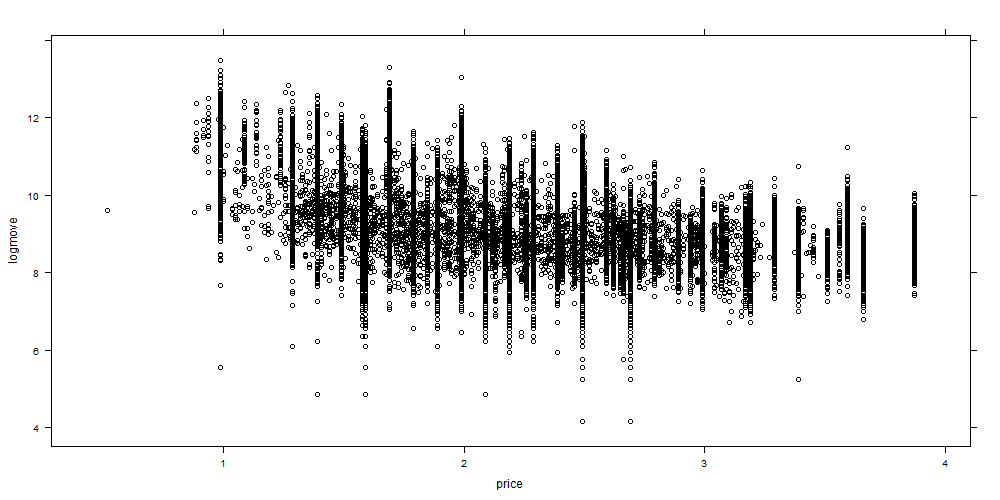
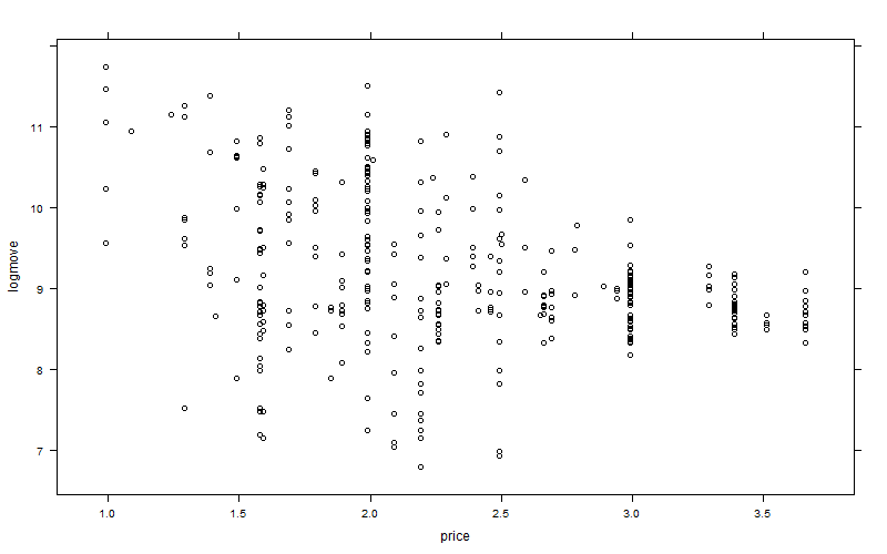
xyplot(logmove~price,data=oj,col="black")
dev.copy(png,'oj_logmoveprice.png',width = 1000, height = 500)
dev.off()
#---------------------------------
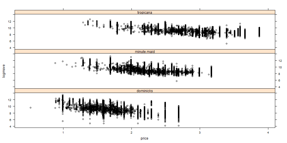
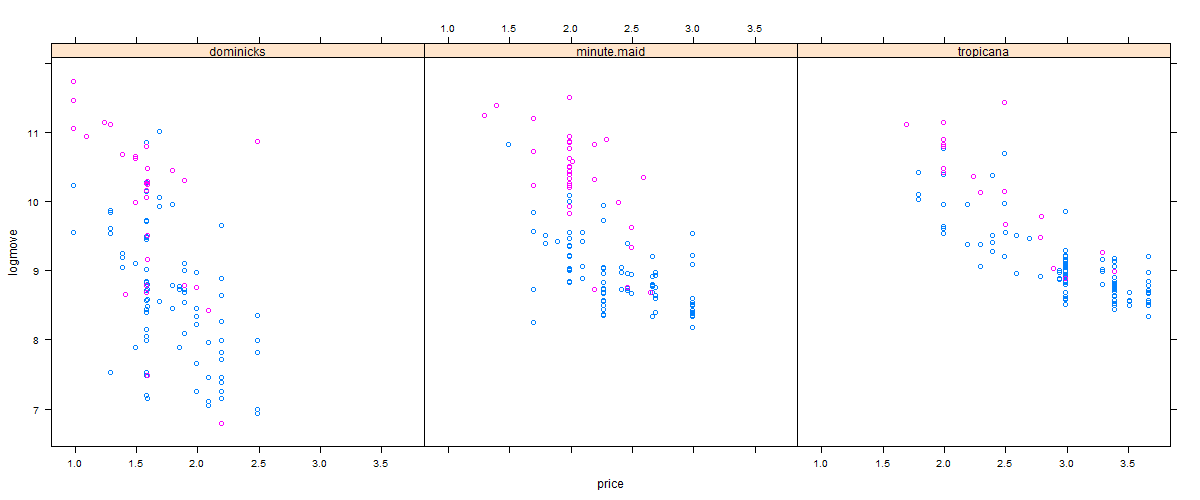
xyplot(logmove~price|brand,data=oj,layout=c(1,3),col="black")
dev.copy(png,'oj_logmovepricebrand.png',width = 1000, height = 500)
dev.off()
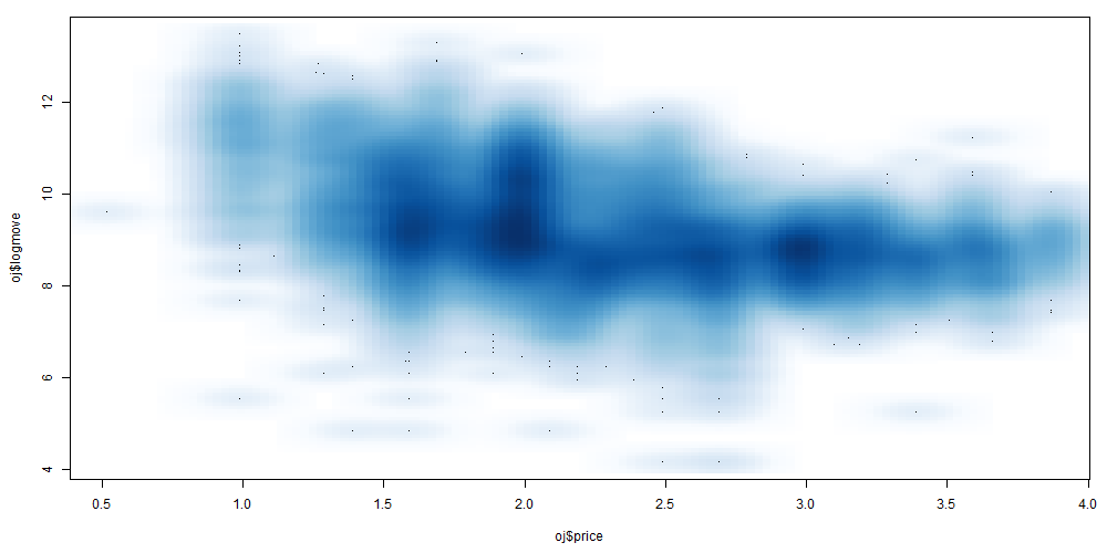
#---------------------------------
smoothScatter(oj$price,oj$logmove)
dev.copy(png,'oj_logmovepricesmooth.png',width = 1000, height = 500)
dev.off()
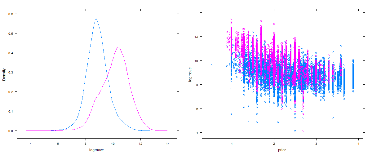
#---------------------------------
a1=densityplot(~logmove,groups=feat, data=oj, plot.points=FALSE)
a2=xyplot(logmove~price,groups=feat, data=oj)
grid.arrange(a1, a2, ncol = 2) #display the two plot a and p
dev.copy(png,'oj_logmovepricegroupfeat.png',width = 1200, height = 500)
dev.off()
#------------------------------------------------
oj1=oj[oj$store == 5,]
xyplot(logmove~week|brand,data=oj1,type="l",layout=c(1,3),col="black")
dev.copy(png,'oj_logmovebrand.png',width = 1200, height = 500)
dev.off()
xyplot(logmove~price,data=oj1,col="black")
dev.copy(png,'oj_logmovepricexyplot.png',width = 800, height = 500)
dev.off()
xyplot(logmove~price|brand,data=oj1,layout=c(1,3),col="black")
dev.copy(png,'oj_logmovepricebrandxyplot.png',width = 1000, height = 500)
dev.off()
densityplot(~logmove|brand,groups=feat,data=oj1,plot.points=FALSE)
dev.copy(png,'oj_logmovebranddenst.png',width = 1200, height = 500)
dev.off()
xyplot(logmove~price|brand,groups=feat,data=oj1)
dev.copy(png,'oj_logmovepricebrandxyplot.png',width = 1200, height = 500)
dev.off()
#----------------------------
t21=tapply(oj$INCOME,oj$store,FUN=mean,na.rm=TRUE)
t21
t21[t21==max(t21)]
t21[t21==min(t21)]
oj1=oj[oj$store == 62,]
oj2=oj[oj$store == 75,]
oj3=rbind(oj1,oj2)
#----------------------------------------
a1=xyplot(logmove~price|store,data=oj3)
a2=xyplot(logmove~price|store,groups=feat,data=oj3)
grid.arrange(a1, a2, ncol = 1) #display the two plot a and p
dev.copy(png,'oj_logmovexyplotprice.png',width = 500, height = 1000)
dev.off()
## store in the wealthiest neighborhood
plot.new()
par(mar=c(4,4,1,1)+0.1,mfrow=c(1,2),bg="white",cex = 1, cex.main = 1)
mhigh=lm(logmove~price,data=oj1)
summary(mhigh)
plot(logmove~price,data=oj1,xlim=c(0,4),ylim=c(0,13), main="62 = wealthiest store")
abline(mhigh)
## store in the poorest neighborhood
mlow=lm(logmove~price,data=oj2)
summary(mlow)
plot(logmove~price,data=oj2,xlim=c(0,4),ylim=c(0,13), main="75 = poorest store")
abline(mlow)
dev.copy(png,'oj_logmovepriceoj2.png',width = 1000, height = 300)
dev.off()
Graphs
Mean of logmove over 121 weeks
boxplot
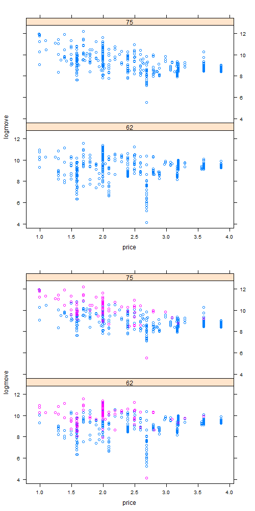
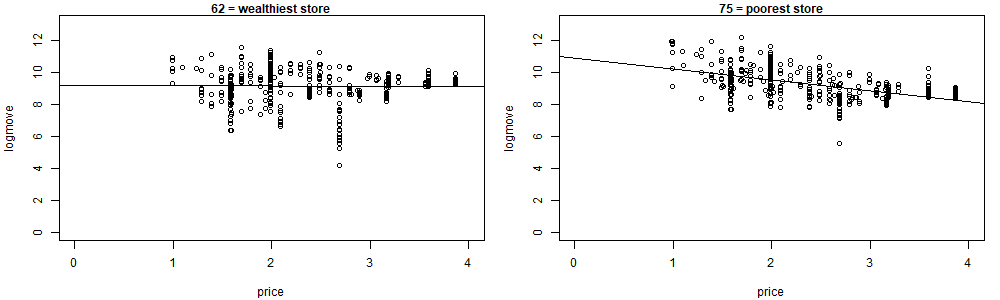
The last two graphs also present the regression lines with summary of coefficients using lm function
mhigh=lm(logmove~price,data=oj1)
summary(mhigh)
Call:
lm(formula = logmove ~ price, data = oj1)
Residuals:
Min 1Q Median 3Q Max
-4.9557 -0.4934 0.1815 0.6557 2.4454
Coefficients:
Estimate Std. Error t value Pr(>|t|)
(Intercept) 9.15394 0.21112 43.359 <2e-16 ***
price -0.01461 0.08381 -0.174 0.862
---
Signif. codes: 0 ‘***’ 0.001 ‘**’ 0.01 ‘*’ 0.05 ‘.’ 0.1 ‘ ’ 1
Residual standard error: 1.142 on 349 degrees of freedom
Multiple R-squared: 8.712e-05, Adjusted R-squared: -0.002778
F-statistic: 0.03041 on 1 and 349 DF, p-value: 0.8617
mlow=lm(logmove~price,data=oj2)
summary(mlow)
Call:
lm(formula = logmove ~ price, data = oj2)
Residuals:
Min 1Q Median 3Q Max
-3.5235 -0.5606 0.0392 0.5090 2.4523
Coefficients:
Estimate Std. Error t value Pr(>|t|)
(Intercept) 10.87695 0.15184 71.63 <2e-16 ***
price -0.67222 0.06071 -11.07 <2e-16 ***
---
Signif. codes: 0 ‘***’ 0.001 ‘**’ 0.01 ‘*’ 0.05 ‘.’ 0.1 ‘ ’ 1
Residual standard error: 0.8383 on 352 degrees of freedom
Multiple R-squared: 0.2584, Adjusted R-squared: 0.2563
F-statistic: 122.6 on 1 and 352 DF, p-value: < 2.2e-16
Nam Le
Risk and Asset Management Specialist for Buildings and Engineering Systems
My research interests include Operation Research and Applied Statistics for Asset Management of Buildings and Engineering Systems.