Return on Investment (ROI) for Intervention of Pumps under uncertainties
This post describes a generic approach on the computation of Net Present Value (NPV) and Life Cycle Cost estimation (LCC) for Preventive Intervention (PI) on pumps (e.g. centrifugal pumps) when decision makers are uncertain on, or do not have a rich set of data on failure of pump components.
Ideally, failure data on pump components should be recorded in time-series fashion that allows analyst to investigate on the frequency of failure and come up with a prediction. The prediction is powerful in view of generating budget for purchasing spare parts for not only one pump station but also for the entire network of pump stations. This is so-called Integrated Asset Management approach that should be at the center of an organization who has a long term view on how to sustain and prolong their assets.
However, in many practical situations, failure data is limited or recorded inappropriately that does not become a useful set of information for analytic. In such a circumstance, decisions on whether to replace/rehabilitate pumps should be dependent on various uncertainty factors such as efficiency, assumption on average decaying rate of the assets, and most importantly the energy consumption vs the production produce.
This article presents a simple yet useful model for managers to make decisions on replacement of pumps if they are more or less aware of deficiency, low efficiency, and high ratio of energy and production over time.
Aside from the above, it is also worth to consider replacement of pumps when the two following aspects are existed.
- Asset obsolescence;
- Technological innovation.
There two aspects should be viewed in a combination. Asset obsolescence could be a result of technological innovation or changes in standards and requirements. Suffice it to state that pumps of a station were designed/installed more than a decade ago, nowadays, pumps are designed and manufactured to be more reliable and durable, whilst the capital cost is significant lower than that in the past.
The model
Total Cost (TC) incurred in a period of T years is defined as the summation of Capital Cost (C) and Operation cost (O). It is note that operational cost includes routine maintenance cost.
$$ TC(T) = \sum_{i=1}^{I} \sum_{t=1}^{T}\frac{C_{i,t}+O_{i,t}\times \epsilon_{i,t}^{new}\times u_{i,t}+(1-\delta_{i,t})\times O_{i,t}\epsilon_{i,t}^{old}\times u_{i,t}}{(1+\rho)^t}$$
In the equation, $\epsilon_{i,t}$, $u_{i,t}$, and $\delta_{i,t}$ are the decreasing rate of efficiency, utilization, and decision variable of pump i in year t, respectively.
Example
A pump station has 6 booster pumps with the same configuration of 500 horsepower. The station has been in commission for more than 10 years and there has been a progressive degradation process, though it has not been captured appropriately. Sufficient failure data at component level is not available.
Tests have been conducted to measure the flow and the power rating that allows to come up efficiency of pump. However, due to non-optimal pipe configuration, the obtained efficiencies are also subjected to uncertainties.
Under such circumstance, decision makers have to make decisions under uncertainties.
- Discount factor is 8.5% annually;
- Capital cost for buying/installing a new pump of 500 horsepower would cost 5 millions Peso (~10,000 usd);
- Efficiency of existing pumps are about 5% less than that of the original design;
- Pumps are assumed to operate at 98% utilization level;
- Price of 1 KW is 6.5 Peso;
- There are 2 Intervention Strategies (IS) to be considerred. Herein refer to TC1 and TC2, respectively. TC1 is to replace existing pump with a new one in a step of 1 year. TC2 is Do Nothing, i.e., to keep the existing pumps as they are.
Source Code
#this subroutine is used to estimate the cashflow of an investment for pump stations
Npumps = 6 #total number of pumps
TPeriod=10 #this infers 5 years
TC1<-matrix(nrow=TPeriod,ncol = Npumps) #Option 1
TC2<-matrix(nrow=TPeriod,ncol = Npumps) #Option 2
CAPEX<-matrix(nrow=TPeriod,ncol = Npumps) #Captical investment cost
OPEX<-matrix(nrow=TPeriod,ncol = Npumps) #Operational Cost
delta<-matrix(nrow=TPeriod,ncol = Npumps) #decrease in efficiency
epsilonold<-matrix(nrow=TPeriod,ncol = Npumps) #decrease in efficiency
epsilonnew<-matrix(nrow=TPeriod,ncol = Npumps) #decrease in efficiency
u<-matrix(nrow=TPeriod,ncol = Npumps) #ultilization
rho=0.085 #discount factor
pricee=6.5
hoursepower=500
utilization=0.98
Newpumpcost=5000000
#Option 1 - Stagging investment for pump
for (t in 1: TPeriod){
if (t<2){
for (i in 1:Npumps){
epsilonold[t,i]<-1.05
}
} else {
for (i in 1:Npumps){
epsilonold[t,i]<-epsilonold[t-1,i]*1.05
}
}
}
for (t in 1:TPeriod){
for (i in 1:Npumps){
delta[,]<-0
delta[1,1]<-1
epsilonnew[1,1]<-1
delta[2,2]<-1
epsilonnew[2,2]<-1
delta[3,3]<-1
epsilonnew[3,3]<-1
delta[4,4]<-1
epsilonnew[4,4]<-1
delta[5,5]<-1
epsilonnew[5,5]<-1
delta[6,6]<-1
epsilonnew[6,6]<-1
CAPEX[t,i]<-Newpumpcost #peso
u[t,i]<-utilization
OPEX[t,i]<- pricee*hoursepower*365*24*0.746*u[t,i] #peso
}
}
for (t in 1: TPeriod){
for (i in 1:Npumps){
if (delta[t,i]==1){
epsilonnew[t,i]<-1
} else if (i==1 & t==1){
epsilonnew[t,i]<-1
} else if (t>1){
epsilonnew[t,i]<-epsilonnew[t-1,i]*1
}
}
}
epsilonnew[is.na(epsilonnew)] <- 0
#redefine the value of epsilonold based on new value of epsilonnew
for (t in 1: TPeriod){
for (i in 1:Npumps){
if (epsilonnew[t,i]<1){
epsilonold[t,i]<-epsilonold[t,i]
} else if (epsilonnew[t,i]==1){
epsilonold[t,i]<-0
}
}
}
for (i in 1:Npumps){
for (t in 1:TPeriod){
TC1[t,i]<-(((CAPEX[t,i]*delta[t,i]+OPEX[t,i]*epsilonnew[t,i]))+(1-delta[t,i])*OPEX[t,i]*epsilonold[t,i])/(1+rho)**t
}
}
cat("Replacement of pumps \n")
print(TC1)
#stop("dd")
#Option 2 - Do Nothing
for (t in 1:TPeriod){
for (i in 1:Npumps){
delta[,]<-0
CAPEX[t,i]<-0 #peso
u[t,i]<-utilization
epsilonnew[t,i]<-1.0
OPEX[t,i]<- pricee*hoursepower*365*24*0.746*u[t,i] #peso
}
}
for (t in 1: TPeriod){
if (t<2){
for (i in 1:Npumps){
epsilonold[t,i]<-1.05
}
} else {
for (i in 1:Npumps){
epsilonold[t,i]<-epsilonold[t-1,i]*1.05
}
}
}
for (i in 1:Npumps){
for (t in 1:TPeriod){
TC2[t,i]<-(((CAPEX[t,i]+OPEX[t,i]*epsilonnew[t,i])*delta[t,i])+(1-delta[t,i])*OPEX[t,i]*epsilonold[t,i])/(1+rho)**t
}
}
cat("Do Nothing \n")
print(TC2)
cat("The difference of investment \n")
print(TC1-TC2)
#plot the graph for comparison
library(ggplot2)
time=c(1:TPeriod)
x<-data.frame(dat=TC1[,1],IS=rep("TC1"))
y<-data.frame(dat=TC2[,1],IS=rep("TC2"))
x<-cbind(time,x)
y<-cbind(time,y)
xy<- rbind(x, y)
ggplot(xy, aes(fill=IS, y=dat, x=factor(time))) + geom_bar(position="dodge", stat="identity")
stop("")
TC1<-data.frame(TC1,IS=rep("TC1"))
TC2<-data.frame(TC2,IS=rep("TC2"))
#TC2<-data.frame(TC2=TC2[,1])
#TC1<-data.frame(TC1)
#TC2<-data.frame(TC2)
TC1<-cbind(time,TC1)
TC2<-cbind(time,TC2)
library(reshape)
mdataTC1 <- melt(TC1,id=c("time","IS"))
mdataTC2 <- melt(TC2,id=c("time","IS"))
#joint the two data
total <- rbind(mdataTC1, mdataTC2)
ggplot(total, aes(fill=IS, y=value, x=factor(time)),variable=X1) + geom_bar(position="dodge", stat="identity")
#ggplot(total, aes(fill=variable, y=value, x=factor(time)),variable=X1) + geom_bar(position="fill", stat="identity")
#ggplot(total, aes(y=value, x=variable, color=IS, fill=IS)) + geom_bar( stat="identity") + facet_wrap(~factor(time))
Results
Estimation results are shown in following tables
source(‘C:/Dropbox/workspace/RProjects/PlantAudit/PAG/tc.R’) Replacement of pumps
          [,1]     [,2]     [,3]     [,4]     [,5]     [,6]
 [1,] 23791565 20142433 20142433 20142433 20142433 20142433
 [2,] 17680433 21927709 19492677 19492677 19492677 19492677
 [3,] 16295330 16295330 20209870 18863881 18863881 18863881
 [4,] 15018737 15018737 15018737 18626609 18255369 18255369
 [5,] 13842154 13842154 13842154 13842154 17167381 17666486
 [6,] 12757746 12757746 12757746 12757746 12757746 15822471
 [7,] 11758291 11758291 11758291 11758291 11758291 11758291
 [8,] 10837135 10837135 10837135 10837135 10837135 10837135
 [9,]  9988142  9988142  9988142  9988142  9988142  9988142
[10,]  9205661  9205661  9205661  9205661  9205661  9205661
Do Nothing
          [,1]     [,2]     [,3]     [,4]     [,5]     [,6]
 [1,] 20142433 20142433 20142433 20142433 20142433 20142433
 [2,] 19492677 19492677 19492677 19492677 19492677 19492677
 [3,] 18863881 18863881 18863881 18863881 18863881 18863881
 [4,] 18255369 18255369 18255369 18255369 18255369 18255369
 [5,] 17666486 17666486 17666486 17666486 17666486 17666486
 [6,] 17096599 17096599 17096599 17096599 17096599 17096599
 [7,] 16545096 16545096 16545096 16545096 16545096 16545096
 [8,] 16011383 16011383 16011383 16011383 16011383 16011383
 [9,] 15494887 15494887 15494887 15494887 15494887 15494887
[10,] 14995052 14995052 14995052 14995052 14995052 14995052
The difference of investment
          [,1]     [,2]     [,3]       [,4]       [,5]     [,6]
 [1,]  3649131        0        0        0.0        0.0        0
 [2,] -1812244  2435032        0        0.0        0.0        0
 [3,] -2568551 -2568551  1345989        0.0        0.0        0
 [4,] -3236632 -3236632 -3236632   371239.7        0.0        0
 [5,] -3824332 -3824332 -3824332 -3824332.0  -499104.8        0
 [6,] -4338854 -4338854 -4338854 -4338853.7 -4338853.7 -1274128
 [7,] -4786805 -4786805 -4786805 -4786805.2 -4786805.2 -4786805
 [8,] -5174249 -5174249 -5174249 -5174248.9 -5174248.9 -5174249
 [9,] -5506745 -5506745 -5506745 -5506744.7 -5506744.7 -5506745
[10,] -5789391 -5789391 -5789391 -5789390.9 -5789390.9 -5789391
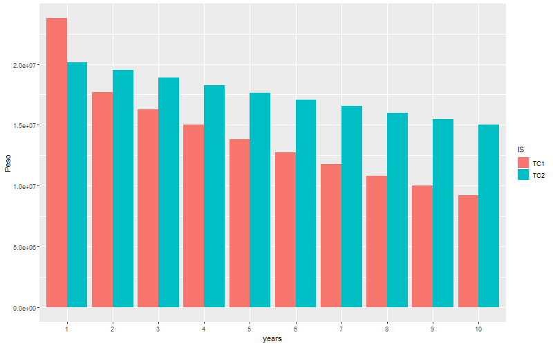
As can be seen from the table of difference, if pump 1 is to be replaced (TC1) now (year 1), the Owner needs to spend 5 millions Peso for the pump, plus the energy cost for that year, the total cost in year 1 would be 23,791,565 Peso. Meanwhile, if pump 1 is to follow TC2 (Do Nothing), there is a cost of 20,142,433 Peso, which is basically the energy cost. The difference between TC1 and TC2 in year 1 is 3,649,131 Peso, meaning the Owner will spend more money in year 1. In other words, there is a negative cash flow in the first year.
However, from 2nd year onward, there is a decreasing in energy consumption, this is thanks to the higher efficiency pump that consume less energy. As a result, there is a saving of -1,812,244 Peso. This value has been discounted and it is the Net Present Value of the OPEX incurred in year two. This difference can be notably seen in the following graph. This graph clearly shows that more energy in following years will be saved if the pump 1 is to be replaced now. It can also be dictated that the amount of cost associated with the saving in energy will compensate the CAPEX within 2 years of investment.
Nam Le
Risk and Asset Management Specialist for Buildings and Engineering Systems
My research interests include Operation Research and Applied Statistics for Asset Management of Buildings and Engineering Systems.