Fuel Efficiency - Regression Analysis
Data Mining and Business Analytics with R
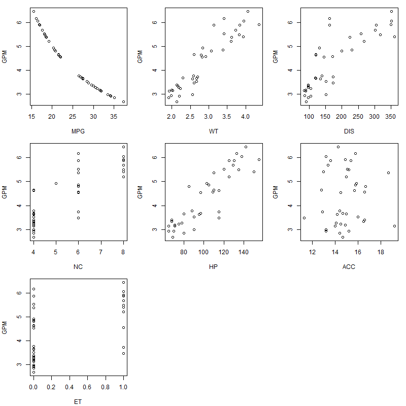
This example shows a very simple regression analysis using fuel data of 38 cars. Code is copied from the book “Data Mining and Business Analytics with R” with minor modification on the graphs.
There are 2 learning points to be remembered with this example.
Leaps package with regsubsets fuction.
Regsubsets function allows to perform regression on subsets of data, particularly useful to compare across model’s predictors to understand the fit of the model.
https://www.rdocumentation.org/packages/leaps/versions/2.1-1/topics/regsubsets
Cross-Validation
Cross-validation removes one case from the data set of n cases, fits the model to the reduced data set, and predicts the response of that one case that has been removed from the estimation. This is repeated for each of the n cases. The summary statistics of the n genuine out-of-sample prediction errors (mean error, root mean square error, mean absolute percent error) help us assess the out-of-sample prediction performance. Cross-validation is very informative as it evaluates the model on new data. We find that the model with all six regressors performs better. It leads to a mean absolute percent error of about 6.75% (as compared to 8.23% for the model with weight as the only regressor).
> FuelEff
    GPM    WT DIS NC  HP  ACC ET
1  5.917 4.360 350  8 155 14.9  1
2  6.452 4.054 351  8 142 14.3  1
3  5.208 3.605 267  8 125 15.0  1
4  5.405 3.940 360  8 150 13.0  1
5  3.333 2.155  98  4  68 16.5  0
6  3.636 2.560 134  4  95 14.2  0
7  3.676 2.300 119  4  97 14.7  0
8  3.236 2.230 105  4  75 14.5  0
9  4.926 2.830 131  5 103 15.9  0
10 5.882 3.140 163  6 125 13.6  0
11 4.630 2.795 121  4 115 15.7  0
12 6.173 3.410 163  6 133 15.8  0
13 4.854 3.380 231  6 105 15.8  0
14 4.808 3.070 200  6  85 16.7  0
15 5.376 3.620 225  6 110 18.7  0
16 5.525 3.410 258  6 120 15.1  0
17 5.882 3.840 305  8 130 15.4  1
18 5.682 3.725 302  8 129 13.4  1
19 6.061 3.955 351  8 138 13.2  1
20 5.495 3.830 318  8 135 15.2  1
21 3.774 2.585 140  4  88 14.4  0
22 4.566 2.910 171  6 109 16.6  1
23 2.933 1.975  86  4  65 15.2  0
24 2.849 1.915  98  4  80 14.4  0
25 3.650 2.670 121  4  80 15.0  0
26 3.175 1.990  89  4  71 14.9  0
27 3.390 2.135  98  4  68 16.6  0
28 3.521 2.670 151  4  90 16.0  0
29 3.472 2.595 173  6 115 11.3  1
30 3.731 2.700 173  6 115 12.9  1
31 2.985 2.556 151  4  90 13.2  0
32 2.924 2.200 105  4  70 13.2  0
33 3.145 2.020  85  4  65 19.2  0
34 2.681 2.130  91  4  69 14.7  0
35 3.279 2.190  97  4  78 14.1  0
36 4.545 2.815 146  6  97 14.5  0
37 4.651 2.600 121  4 110 12.8  0
38 3.135 1.925  89  4  71 14.0  0
CODE
## first we read in the data

FuelEff <- read.csv("https://www.biz.uiowa.edu/faculty/jledolter/DataMining/FuelEfficiency.csv")
#FuelEff <- read.csv("FuelEfficiency.csv")


FuelEff

#----------------------------

plot.new()
#par(mfrow=c(1,1))

par(mar=c(4,4,1,1)+0.1,mfrow=c(3,3),bg="white",cex = 1, cex.main = 1)
plot(GPM~MPG,data=FuelEff)
plot(GPM~WT,data=FuelEff)
plot(GPM~DIS,data=FuelEff)
plot(GPM~NC,data=FuelEff)
plot(GPM~HP,data=FuelEff)
plot(GPM~ACC,data=FuelEff)
plot(GPM~ET,data=FuelEff)

dev.copy(png,'fueleff_xyplot.png',width = 800, height = 800)
dev.off()


FuelEff=FuelEff[-1] #ignore the MPG column

FuelEff

## regression on all data

m1=lm(GPM~.,data=FuelEff)
summary(m1)

cor(FuelEff)

## best subset regression in R

library(leaps)
X=FuelEff[,2:7]
y=FuelEff[,1]

#use the regsubsets function from package leaps to compute regression of the subsets

#https://www.rdocumentation.org/packages/leaps/versions/2.1-1/topics/regsubsets


out=summary(regsubsets(X,y,nbest=2,nvmax=ncol(X)))
tab=cbind(out$which,out$rsq,out$adjr2,out$cp)
tab

m2=lm(GPM~WT,data=FuelEff)
summary(m2)

## cross-validation (leave one out) for the model on all six regressors

n=length(FuelEff$GPM)
diff=dim(n)
percdiff=dim(n)
for (k in 1:n) {
  train1=c(1:n)
  train=train1[train1!=k]
  ## the R expression "train1[train1!=k]" picks from train1 those

  ## elements that are different from k and stores those elements in the

  ## object train.

  ## For k=1, train consists of elements that are different from 1; that

  ## is 2, 3, …, n.

  m1=lm(GPM~.,data=FuelEff[train,])
  pred=predict(m1,newdat=FuelEff[-train,]) #adding the new data, which is ignored earlier

  obs=FuelEff$GPM[-train]
  diff[k]=obs-pred
  percdiff[k]=abs(diff[k])/obs
}
me=mean(diff)
rmse=sqrt(mean(diff**2))
mape=100*(mean(percdiff))
me   # mean error

rmse # root mean square error

mape # mean absolute percent error


## cross-validation (leave one out) for the model on weight only

n=length(FuelEff$GPM)
diff=dim(n)
percdiff=dim(n)
for (k in 1:n) {
  train1=c(1:n)
  train=train1[train1!=k]
  m2=lm(GPM~WT,data=FuelEff[train,])
  pred=predict(m2,newdat=FuelEff[-train,])
  obs=FuelEff$GPM[-train]
  diff[k]=obs-pred
  percdiff[k]=abs(diff[k])/obs
}
me=mean(diff)
rmse=sqrt(mean(diff**2))
mape=100*(mean(percdiff))
me   # mean error

rmse # root mean square error

mape # mean absolute percent error
Graphs and Outcomes
## regression on all data
m1=lm(GPM~.,data=FuelEff)
summary(m1)
Call:
lm(formula = GPM ~ ., data = FuelEff)
Residuals:
Min 1Q Median 3Q Max
-0.4996 -0.2547 0.0402 0.1956 0.6455
Coefficients:
Estimate Std. Error t value Pr(>|t|)
(Intercept) -2.599357 0.663403 -3.918 0.000458 ***
WT 0.787768 0.451925 1.743 0.091222 .
DIS -0.004890 0.002696 -1.814 0.079408 .
NC 0.444157 0.122683 3.620 0.001036 **
HP 0.023599 0.006742 3.500 0.001431 **
ACC 0.068814 0.044213 1.556 0.129757
ET -0.959634 0.266785 -3.597 0.001104 **
---
Signif. codes: 0 ‘***’ 0.001 ‘**’ 0.01 ‘*’ 0.05 ‘.’ 0.1 ‘ ’ 1
Residual standard error: 0.313 on 31 degrees of freedom
Multiple R-squared: 0.9386, Adjusted R-squared: 0.9267
F-statistic: 78.94 on 6 and 31 DF, p-value: < 2.2e-16
cor(FuelEff)
GPM WT DIS NC HP ACC ET
GPM 1.00000000 0.92626656 0.8229098 0.8411880 0.8876992 0.03307093 0.5206121
WT 0.92626656 1.00000000 0.9507647 0.9166777 0.9172204 -0.03357386 0.6673661
DIS 0.82290984 0.95076469 1.0000000 0.9402812 0.8717993 -0.14341745 0.7746636
NC 0.84118805 0.91667774 0.9402812 1.0000000 0.8638473 -0.12924363 0.8311721
HP 0.88769915 0.91722045 0.8717993 0.8638473 1.0000000 -0.25262113 0.7202350
ACC 0.03307093 -0.03357386 -0.1434174 -0.1292436 -0.2526211 1.00000000 -0.3102336
ET 0.52061208 0.66736606 0.7746636 0.8311721 0.7202350 -0.31023357 1.0000000
## best subset regression in R
library(leaps)
X=FuelEff[,2:7]
y=FuelEff[,1]
out=summary(regsubsets(X,y,nbest=2,nvmax=ncol(X)))
tab=cbind(out$which,out$rsq,out$adjr2,out$cp)
tab
(Intercept) WT DIS NC HP ACC ET
1 1 1 0 0 0 0 0 0.8579697 0.8540244 37.674750
1 1 0 0 0 1 0 0 0.7880098 0.7821212 72.979632
2 1 1 1 0 0 0 0 0.8926952 0.8865635 22.150747
2 1 1 0 0 0 0 1 0.8751262 0.8679906 31.016828
3 1 0 0 1 1 0 1 0.9145736 0.9070360 13.109930
3 1 1 1 1 0 0 0 0.9028083 0.8942326 19.047230
4 1 0 0 1 1 1 1 0.9313442 0.9230223 6.646728
4 1 1 0 1 1 0 1 0.9204005 0.9107520 12.169443
5 1 1 1 1 1 0 1 0.9337702 0.9234218 7.422476
5 1 0 1 1 1 1 1 0.9325494 0.9220103 8.038535
6 1 1 1 1 1 1 1 0.9385706 0.9266810 7.000000
m2=lm(GPM~WT,data=FuelEff)
summary(m2)
Call:
lm(formula = GPM ~ WT, data = FuelEff)
Residuals:
Min 1Q Median 3Q Max
-0.88072 -0.29041 0.00659 0.19021 1.13164
Coefficients:
Estimate Std. Error t value Pr(>|t|)
(Intercept) -0.006101 0.302681 -0.02 0.984
WT 1.514798 0.102721 14.75 <2e-16 ***
---
Signif. codes: 0 ‘***’ 0.001 ‘**’ 0.01 ‘*’ 0.05 ‘.’ 0.1 ‘ ’ 1
Residual standard error: 0.4417 on 36 degrees of freedom
Multiple R-squared: 0.858, Adjusted R-squared: 0.854
F-statistic: 217.5 on 1 and 36 DF, p-value: < 2.2e-16
Nam Le
Risk and Asset Management Specialist for Buildings and Engineering Systems
My research interests include Operation Research and Applied Statistics for Asset Management of Buildings and Engineering Systems.