Price of 2nd hand Toyota cars - Regression Analysis
Data Mining and Business Analytics with R
This example shows another very simple regression analysis using data of secondhand Toyota car prices. Code is copied from the book “Data Mining and Business Analytics with R” with minor modification on the graphs.
The regressions are done treating Price of Cars as functions of predictors such as Car weight, Model types, Number of cylinders, etc.
Focus is on: (1) Select a trained set of data that gives Mean Error close to 0 as possible; (2) Cross Validate the data to provide an insight on better Predictors to be used in the model.
Data.
#toyota <- read.csv("ToyotaCorolla.csv")

toyota[1:3,]
  Price Age    KM FuelType HP MetColor Automatic   CC Doors Weight
1 13500  23 46986   Diesel 90        1         0 2000     3   1165
2 13750  23 72937   Diesel 90        1         0 2000     3   1165
3 13950  24 41711   Diesel 90        1         0 2000     3   1165
CODE
## first we read in the data
toyota <- read.csv("https://www.biz.uiowa.edu/faculty/jledolter/DataMining/ToyotaCorolla.csv")
#toyota <- read.csv("ToyotaCorolla.csv")
toyota[1:3,]
summary(toyota)
hist(toyota$Price)
## next we create indicator variables for the categorical variable
## FuelType with its three nominal outcomes: CNG, Diesel, and Petrol
v1=rep(1,length(toyota$FuelType))
v2=rep(0,length(toyota$FuelType))
toyota$FuelType1=ifelse(toyota$FuelType=="CNG",v1,v2) #return value of CNG to v1, otherwise 0
toyota$FuelType2=ifelse(toyota$FuelType=="Diesel",v1,v2) #return value of Diesel to v1, otherwise 0
auto=toyota[-4] #ignore column 4 (Fueltype)
auto[1:3,]
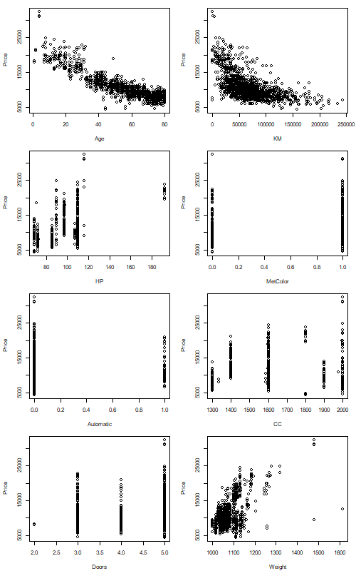
plot.new()
#par(mfrow=c(1,1))
par(mar=c(4,4,1,1)+0.1,mfrow=c(4,2),bg="white",cex = 0.7, cex.main = 1)
plot(Price~Age,data=auto)
plot(Price~KM,data=auto)
plot(Price~HP,data=auto)
plot(Price~MetColor,data=auto)
plot(Price~Automatic,data=auto)
plot(Price~CC,data=auto)
plot(Price~Doors,data=auto)
plot(Price~Weight,data=auto)
dev.copy(png,'toyota_xyplot.png',width = 500, height = 800)
dev.off()
## regression on all data
m1=lm(Price~.,data=auto)
summary(m1)
set.seed(1)
## fixing the seed value for the random selection guarantees the
## same results in repeated runs
n=length(auto$Price)
n1=1000
n2=n-n1
train=sample(1:n,n1) # generate random n1 integer number of data among the size from 1 to n.
## regression on training set
m1=lm(Price~.,data=auto[train,])
summary(m1)
pred=predict(m1,newdat=auto[-train,]) #adding a set of n2 number into regression model
obs=auto$Price[-train]
diff=obs-pred
percdiff=abs(diff)/obs
me=mean(diff)
rmse=sqrt(sum(diff**2)/n2)
mape=100*(mean(percdiff))
me # mean error
rmse # root mean square error
mape # mean absolute percent error
## cross-validation (leave one out)
n=length(auto$Price)
diff=dim(n)
percdiff=dim(n)
for (k in 1:n) {
train1=c(1:n)
train=train1[train1!=k]
m1=lm(Price~.,data=auto[train,])
pred=predict(m1,newdat=auto[-train,])
obs=auto$Price[-train]
diff[k]=obs-pred
percdiff[k]=abs(diff[k])/obs
}
me=mean(diff)
rmse=sqrt(mean(diff**2))
mape=100*(mean(percdiff))
me # mean error
rmse # root mean square error
mape # mean absolute percent error
## cross-validation (leave one out): Model with just Age
n=length(auto$Price)
diff=dim(n)
percdiff=dim(n)
for (k in 1:n) {
train1=c(1:n)
train=train1[train1!=k]
m1=lm(Price~Age,data=auto[train,])
pred=predict(m1,newdat=auto[-train,])
obs=auto$Price[-train]
diff[k]=obs-pred
percdiff[k]=abs(diff[k])/obs
}
me=mean(diff)
rmse=sqrt(mean(diff**2))
mape=100*(mean(percdiff))
me # mean error
rmse # root mean square error
mape # mean absolute percent error
## Adding the squares of Age and KM to the model
auto$Age2=auto$Age^2
auto$KM2=auto$KM^2
m11=lm(Price~Age+KM,data=auto)
summary(m11)
m12=lm(Price~Age+Age2+KM+KM2,data=auto)
summary(m12)
m13=lm(Price~Age+Age2+KM,data=auto)
summary(m13)
#----------------
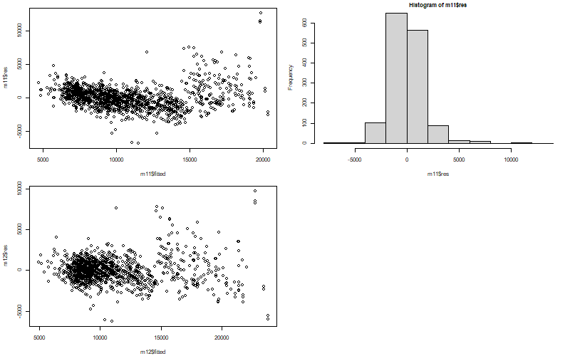
plot.new()
#par(mfrow=c(1,1))
par(mar=c(4,4,1,1)+0.1,mfrow=c(2,2),bg="white",cex = 0.7, cex.main = 1)
plot(m11$res~m11$fitted)
hist(m11$res)
plot(m12$res~m12$fitted)
dev.copy(png,'toyota_m11m12.png',width = 800, height = 500)
dev.off()
Graphs and Outcomes
Highlights
Function ifelse() is used to return the logical value YES or NO.
## next we create indicator variables for the categorical variable

## FuelType with its three nominal outcomes: CNG, Diesel, and Petrol

v1=rep(1,length(toyota$FuelType))
v2=rep(0,length(toyota$FuelType))
toyota$FuelType1=ifelse(toyota$FuelType=="CNG",v1,v2) #return value of CNG to v1, otherwise 0

toyota$FuelType2=ifelse(toyota$FuelType=="Diesel",v1,v2) #return value of Diesel to v1, otherwise 0
m1=lm(Price~.,data=auto)
summary(m1)

Call:
lm(formula = Price ~ ., data = auto)

Residuals:
     Min       1Q   Median       3Q      Max
-10642.3   -737.7      3.1    731.3   6451.5

Coefficients:
              Estimate Std. Error t value Pr(>|t|)
(Intercept) -2.681e+03  1.219e+03  -2.199 0.028036 *
Age         -1.220e+02  2.602e+00 -46.889  < 2e-16 ***
KM          -1.621e-02  1.313e-03 -12.347  < 2e-16 ***
HP           6.081e+01  5.756e+00  10.565  < 2e-16 ***
MetColor     5.716e+01  7.494e+01   0.763 0.445738
Automatic    3.303e+02  1.571e+02   2.102 0.035708 *
CC          -4.174e+00  5.453e-01  -7.656 3.53e-14 ***
Doors       -7.776e+00  4.006e+01  -0.194 0.846129
Weight       2.001e+01  1.203e+00  16.629  < 2e-16 ***
FuelType1   -1.121e+03  3.324e+02  -3.372 0.000767 ***
FuelType2    2.269e+03  4.394e+02   5.164 2.75e-07 ***
---
Signif. codes:  0 ‘***’ 0.001 ‘**’ 0.01 ‘*’ 0.05 ‘.’ 0.1 ‘ ’ 1

Residual standard error: 1316 on 1425 degrees of freedom
Multiple R-squared:  0.8693,    Adjusted R-squared:  0.8684
F-statistic:   948 on 10 and 1425 DF,  p-value: < 2.2e-16
set.seed(1)
## fixing the seed value for the random selection guarantees the

## same results in repeated runs

n=length(auto$Price)
n1=1000
n2=n-n1
train=sample(1:n,n1) # generate random n1 integer number of data among the size from 1 to n.


## regression on training set

m1=lm(Price~.,data=auto[train,])
summary(m1)

Call:
lm(formula = Price ~ ., data = auto[train, ])

Residuals:
    Min      1Q  Median      3Q     Max
-8914.6  -778.2   -22.0   751.4  6480.4

Coefficients:
              Estimate Std. Error t value Pr(>|t|)
(Intercept)  5.337e+02  1.417e+03   0.377    0.706
Age         -1.233e+02  3.184e+00 -38.725  < 2e-16 ***
KM          -1.726e-02  1.585e-03 -10.892  < 2e-16 ***
HP           5.472e+01  7.662e+00   7.142 1.78e-12 ***
MetColor     1.581e+02  9.199e+01   1.719    0.086 .
Automatic    2.703e+02  1.982e+02   1.364    0.173
CC          -3.634e+00  7.031e-01  -5.168 2.86e-07 ***
Doors        3.828e+01  4.851e+01   0.789    0.430
Weight       1.671e+01  1.379e+00  12.118  < 2e-16 ***
FuelType1   -5.950e+02  4.366e+02  -1.363    0.173
FuelType2    2.279e+03  5.582e+02   4.083 4.80e-05 ***
---
Signif. codes:  0 ‘***’ 0.001 ‘**’ 0.01 ‘*’ 0.05 ‘.’ 0.1 ‘ ’ 1

Residual standard error: 1343 on 989 degrees of freedom
Multiple R-squared:  0.8573,    Adjusted R-squared:  0.8559
F-statistic: 594.3 on 10 and 989 DF,  p-value: < 2.2e-16
## regression on training set

m1=lm(Price~.,data=auto[train,])
summary(m1)
pred=predict(m1,newdat=auto[-train,]) #adding a set of n2 number into regression model

obs=auto$Price[-train]
diff=obs-pred
percdiff=abs(diff)/obs
me=mean(diff)
rmse=sqrt(sum(diff**2)/n2)
mape=100*(mean(percdiff))
me   # mean error

rmse # root mean square error

mape # mean absolute percent error


> me   # mean error

[1] -48.70784
> rmse # root mean square error

[1] 1283.097
> mape # mean absolute percent error

[1] 9.208957
The above results give quite high value of Mean Errors, indicating a certain level of bias
## cross-validation (leave one out)

n=length(auto$Price)
diff=dim(n)
percdiff=dim(n)
for (k in 1:n) {
  train1=c(1:n)
  train=train1[train1!=k]
  m1=lm(Price~.,data=auto[train,])
  pred=predict(m1,newdat=auto[-train,])
  obs=auto$Price[-train]
  diff[k]=obs-pred
  percdiff[k]=abs(diff[k])/obs
}
me=mean(diff)
rmse=sqrt(mean(diff**2))
mape=100*(mean(percdiff))
me   # mean error

rmse # root mean square error

mape # mean absolute percent error


> me   # mean error

[1] -2.726251
> rmse # root mean square error

[1] 1354.509
> mape # mean absolute percent error

[1] 9.530529
Now, the Mean Error is -2.7, which is a lot better than that of previous model. We can still further improve
## cross-validation (leave one out): Model with just Age

n=length(auto$Price)
diff=dim(n)
percdiff=dim(n)
for (k in 1:n) {
  train1=c(1:n)
  train=train1[train1!=k]
  m1=lm(Price~Age,data=auto[train,])
  pred=predict(m1,newdat=auto[-train,])
  obs=auto$Price[-train]
  diff[k]=obs-pred
  percdiff[k]=abs(diff[k])/obs
}
me=mean(diff)
rmse=sqrt(mean(diff**2))
mape=100*(mean(percdiff))
me   # mean error

rmse # root mean square error

mape # mean absolute percent error


> me   # mean error

[1] 0.6085014
> rmse # root mean square error

[1] 1748.76
> mape # mean absolute percent error

[1] 12.13156
See, the mean value of 0.6 now. Surely better than previous one.
Nam Le
Risk and Asset Management Specialist for Buildings and Engineering Systems
My research interests include Operation Research and Applied Statistics for Asset Management of Buildings and Engineering Systems.