Polynomial Regression – Volcano Eruption
Data Mining and Business Analytics with R
What is Polynomial Regression? and when to use it
There is a good set of internet articles that well describe the Math behind the Polynomial regression. Some of good references can be with the following links
https://en.wikipedia.org/wiki/Local_regression
https://onlinelibrary.wiley.com/doi/10.1002/9781118596289.ch4
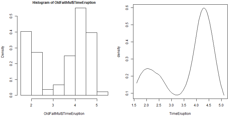
We use polynomial regression in cases when observing histogram, scatter plot, or distribution of data that are not well distributed or clustered into two or more than two groups as shown in below figure.

The plot show that the data points are scattered and seem like the pattern of them follows a sin function. We cannot use linear regression in such as case as linear regression is a straight line function.
Data
Data is from the paper https://onlinelibrary.wiley.com/doi/10.1002/9781118596289.ch4 that includes 272 rows of data on the duration of eruption and waiting time until the next eruption of the Old Faithful volcano.
OldFaithful[1:10,]

TimeEruption TimeWaiting
1         3.600          79
2         1.800          54
3         3.333          74
4         2.283          62
5         4.533          85
6         2.883          55
7         4.700          88
8         3.600          85
9         1.950          51
10        4.350          85
Code
library(locfit)
## first we read in the data
## first we read in the data
#OldFaithful <- read.csv("https://www.biz.uiowa.edu/faculty/jledolter/DataMining/OldFaithful.csv")
OldFaithful <- read.csv("OldFaithful.csv")
OldFaithful[1:10,]
## density histograms and smoothed density histograms
## time of eruption
plot.new()
#par(mfrow=c(1,1))
par(mar=c(4,4,1,1)+0.1,mfrow=c(1,2),bg="white",cex = 1, cex.main = 1)
hist(OldFaithful$TimeEruption,freq=FALSE)
#use locfit https://www.rdocumentation.org/packages/locfit/versions/19980714-2/topics/locfit
fit1 <- locfit(~lp(TimeEruption),data=OldFaithful)
#lp function https://www.rdocumentation.org/packages/lpSolve/versions/5.6.13.1/topics/lp
#lp is a local polynomial model term for Locfit models.
#https://www.rdocumentation.org/packages/locfit/versions/1.5-9.1/topics/lp
plot(fit1)
dev.copy(png,'oldfaithful_timeeruption01.png',width = 800, height = 400)
dev.off()
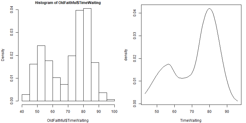
## waiting time to next eruption
hist(OldFaithful$TimeWaiting,freq=FALSE)
fit2 <- locfit(~lp(TimeWaiting),data=OldFaithful)
plot(fit2)
dev.copy(png,'oldfaithful_TimeWaiting01.png',width = 800, height = 400)
dev.off()
#------------------------------
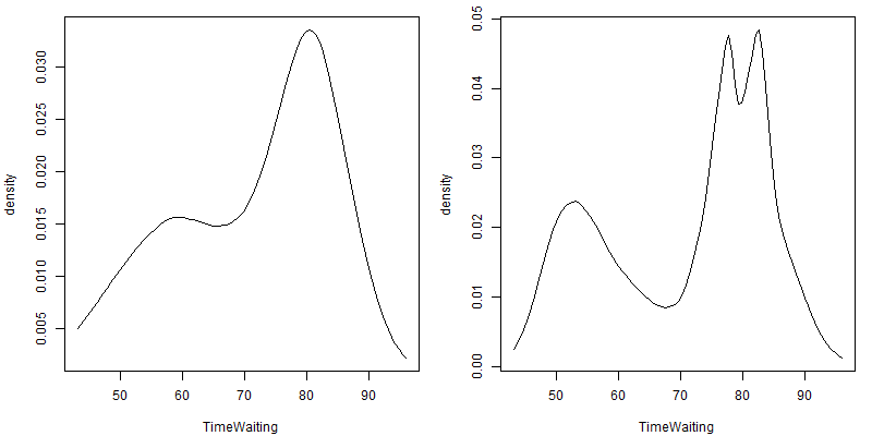
## experiment with different smoothing constants
fit3 <- locfit(~lp(TimeWaiting,nn=0.9,deg=2),data=OldFaithful) #nn is the nearest neighbour component, and deg is the degree of polynomial. default value of nn is 0.6 and deg is 2.
plot(fit3)
fit4 <- locfit(~lp(TimeWaiting,nn=0.3,deg=2),data=OldFaithful)
plot(fit4)
dev.copy(png,'oldfaithful_TimeWaiting02.png',width = 800, height = 400)
dev.off()
## cross-validation of smoothing constant
## for waiting time to next eruption
alpha<-seq(0.20,1,by=0.01)
n1=length(alpha)
g=matrix(nrow=n1,ncol=4)
for (k in 1:length(alpha)) {
g[k,]<-gcv(~lp(TimeWaiting,nn=alpha[k]),data=OldFaithful)
}
g
#gcv is used to estimate the penalty coefficient from the generalized cross-validation criteria. https://www.rdocumentation.org/packages/SpatialExtremes/versions/2.0-7/topics/gcv
plot(g[,4]~g[,3],ylab="GCV",xlab="degrees of freedom")
#the minimum point of the curve indicate the best value of nn. In this case, we can find the minimum value point.
which.min(g[,4])
#This indicate
nn=alpha[which.min(g[,4])] #this is the value of the minimum nn.
fit5 <- locfit(~lp(TimeWaiting,nn=nn,deg=2),data=OldFaithful)
plot(fit5)
dev.copy(png,'oldfaithful_TimeWaiting03.png',width = 800, height = 400)
dev.off()
#------------------------
## local polynomial regression of TimeEruption on TimeWaiting
plot(TimeWaiting~TimeEruption,data=OldFaithful)
# standard regression fit
fitreg=lm(TimeWaiting~TimeEruption,data=OldFaithful)
plot(TimeWaiting~TimeEruption,data=OldFaithful)
abline(fitreg)
dev.copy(png,'oldfaithful_TimeWaitingvseruption01.png',width = 800, height = 400)
dev.off()
#-----------------------------------
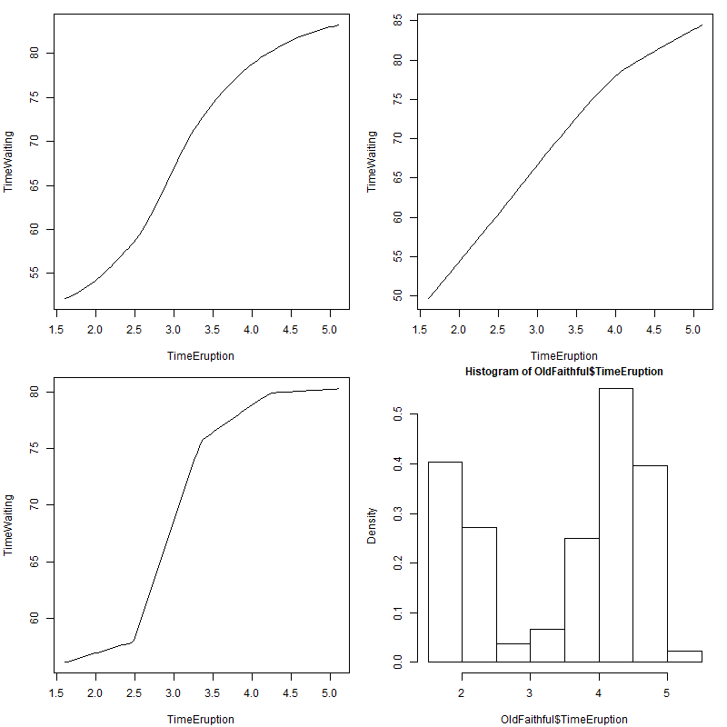
# fit with nearest neighbor bandwidth
plot.new()
#par(mfrow=c(1,1))
par(mar=c(4,4,1,1)+0.1,mfrow=c(2,2),bg="white",cex = 1, cex.main = 1)
fit6 <- locfit(TimeWaiting~lp(TimeEruption),data=OldFaithful)
plot(fit6)
fit7 <- locfit(TimeWaiting~lp(TimeEruption,deg=1),data=OldFaithful)
plot(fit7)
fit8 <- locfit(TimeWaiting~lp(TimeEruption,deg=0),data=OldFaithful)
plot(fit8)
hist(OldFaithful$TimeEruption,freq=FALSE)
dev.copy(png,'oldfaithful_TimeWaitingvseruption02.png',width = 800, height = 800)
dev.off()
Graphs and Highlights
Blow graph shows the minimum points where we can find the best nn value to be used for plotting the right curve.

Part of the code to generate the above 2 graphs is from line 43 to line 61
## cross-validation of smoothing constant

## for waiting time to next eruption

alpha<-seq(0.20,1,by=0.01)
n1=length(alpha)
g=matrix(nrow=n1,ncol=4)
for (k in 1:length(alpha)) {
  g[k,]<-gcv(~lp(TimeWaiting,nn=alpha[k]),data=OldFaithful)
}
g
#gcv is used to estimate the penalty coefficient from the generalized cross-validation criteria. https://www.rdocumentation.org/packages/SpatialExtremes/versions/2.0-7/topics/gcv


plot(g[,4]~g[,3],ylab="GCV",xlab="degrees of freedom")
#the minimum point of the curve indicate the best value of nn. In this case, we can find the minimum value point.

which.min(g[,4])
#This indicate

nn=alpha[which.min(g[,4])] #this is the value of the minimum nn.


fit5 <- locfit(~lp(TimeWaiting,nn=nn,deg=2),data=OldFaithful)
plot(fit5)
Nam Le
Risk and Asset Management Specialist for Buildings and Engineering Systems
My research interests include Operation Research and Applied Statistics for Asset Management of Buildings and Engineering Systems.